lab2

Objetivos¶

• Conhecer algoritmos de classificação, SVM e Randon Forest;

Classificação de digitos 0-9¶

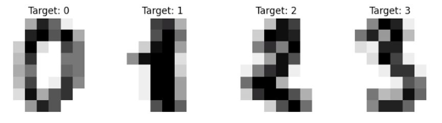
Agora aplicamos os modelos a um dataset mais complexo: reconhecimento de dígitos manuscritos (0-9), com 1797 amostras e 64 features (pixels 8x8).

In [1]:

from sklearn.datasets import load_digits

digits = load_digits()

print(digits)

from sklearn.datasets import load_digits digits = load_digits() print(digits)

{'data': array([[ 0.,  0.,  5., ...,  0.,  0.,  0.],
       [ 0.,  0.,  0., ..., 10.,  0.,  0.],
       [ 0.,  0.,  0., ..., 16.,  9.,  0.],
       ...,
       [ 0.,  0.,  1., ...,  6.,  0.,  0.],
       [ 0.,  0.,  2., ..., 12.,  0.,  0.],
       [ 0.,  0., 10., ..., 12.,  1.,  0.]], shape=(1797, 64)), 'target': array([0, 1, 2, ..., 8, 9, 8], shape=(1797,)), 'frame': None, 'feature_names': ['pixel_0_0', 'pixel_0_1', 'pixel_0_2', 'pixel_0_3', 'pixel_0_4', 'pixel_0_5', 'pixel_0_6', 'pixel_0_7', 'pixel_1_0', 'pixel_1_1', 'pixel_1_2', 'pixel_1_3', 'pixel_1_4', 'pixel_1_5', 'pixel_1_6', 'pixel_1_7', 'pixel_2_0', 'pixel_2_1', 'pixel_2_2', 'pixel_2_3', 'pixel_2_4', 'pixel_2_5', 'pixel_2_6', 'pixel_2_7', 'pixel_3_0', 'pixel_3_1', 'pixel_3_2', 'pixel_3_3', 'pixel_3_4', 'pixel_3_5', 'pixel_3_6', 'pixel_3_7', 'pixel_4_0', 'pixel_4_1', 'pixel_4_2', 'pixel_4_3', 'pixel_4_4', 'pixel_4_5', 'pixel_4_6', 'pixel_4_7', 'pixel_5_0', 'pixel_5_1', 'pixel_5_2', 'pixel_5_3', 'pixel_5_4', 'pixel_5_5', 'pixel_5_6', 'pixel_5_7', 'pixel_6_0', 'pixel_6_1', 'pixel_6_2', 'pixel_6_3', 'pixel_6_4', 'pixel_6_5', 'pixel_6_6', 'pixel_6_7', 'pixel_7_0', 'pixel_7_1', 'pixel_7_2', 'pixel_7_3', 'pixel_7_4', 'pixel_7_5', 'pixel_7_6', 'pixel_7_7'], 'target_names': array([0, 1, 2, 3, 4, 5, 6, 7, 8, 9]), 'images': array([[[ 0.,  0.,  5., ...,  1.,  0.,  0.],
        [ 0.,  0., 13., ..., 15.,  5.,  0.],
        [ 0.,  3., 15., ..., 11.,  8.,  0.],
        ...,
        [ 0.,  4., 11., ..., 12.,  7.,  0.],
        [ 0.,  2., 14., ..., 12.,  0.,  0.],
        [ 0.,  0.,  6., ...,  0.,  0.,  0.]],

       [[ 0.,  0.,  0., ...,  5.,  0.,  0.],
        [ 0.,  0.,  0., ...,  9.,  0.,  0.],
        [ 0.,  0.,  3., ...,  6.,  0.,  0.],
        ...,
        [ 0.,  0.,  1., ...,  6.,  0.,  0.],
        [ 0.,  0.,  1., ...,  6.,  0.,  0.],
        [ 0.,  0.,  0., ..., 10.,  0.,  0.]],

       [[ 0.,  0.,  0., ..., 12.,  0.,  0.],
        [ 0.,  0.,  3., ..., 14.,  0.,  0.],
        [ 0.,  0.,  8., ..., 16.,  0.,  0.],
        ...,
        [ 0.,  9., 16., ...,  0.,  0.,  0.],
        [ 0.,  3., 13., ..., 11.,  5.,  0.],
        [ 0.,  0.,  0., ..., 16.,  9.,  0.]],

       ...,

       [[ 0.,  0.,  1., ...,  1.,  0.,  0.],
        [ 0.,  0., 13., ...,  2.,  1.,  0.],
        [ 0.,  0., 16., ..., 16.,  5.,  0.],
        ...,
        [ 0.,  0., 16., ..., 15.,  0.,  0.],
        [ 0.,  0., 15., ..., 16.,  0.,  0.],
        [ 0.,  0.,  2., ...,  6.,  0.,  0.]],

       [[ 0.,  0.,  2., ...,  0.,  0.,  0.],
        [ 0.,  0., 14., ..., 15.,  1.,  0.],
        [ 0.,  4., 16., ..., 16.,  7.,  0.],
        ...,
        [ 0.,  0.,  0., ..., 16.,  2.,  0.],
        [ 0.,  0.,  4., ..., 16.,  2.,  0.],
        [ 0.,  0.,  5., ..., 12.,  0.,  0.]],

       [[ 0.,  0., 10., ...,  1.,  0.,  0.],
        [ 0.,  2., 16., ...,  1.,  0.,  0.],
        [ 0.,  0., 15., ..., 15.,  0.,  0.],
        ...,
        [ 0.,  4., 16., ..., 16.,  6.,  0.],
        [ 0.,  8., 16., ..., 16.,  8.,  0.],
        [ 0.,  1.,  8., ..., 12.,  1.,  0.]]], shape=(1797, 8, 8)), 'DESCR': ".. _digits_dataset:\n\nOptical recognition of handwritten digits dataset\n--------------------------------------------------\n\n**Data Set Characteristics:**\n\n:Number of Instances: 1797\n:Number of Attributes: 64\n:Attribute Information: 8x8 image of integer pixels in the range 0..16.\n:Missing Attribute Values: None\n:Creator: E. Alpaydin (alpaydin '@' boun.edu.tr)\n:Date: July; 1998\n\nThis is a copy of the test set of the UCI ML hand-written digits datasets\nhttps://archive.ics.uci.edu/ml/datasets/Optical+Recognition+of+Handwritten+Digits\n\nThe data set contains images of hand-written digits: 10 classes where\neach class refers to a digit.\n\nPreprocessing programs made available by NIST were used to extract\nnormalized bitmaps of handwritten digits from a preprinted form. From a\ntotal of 43 people, 30 contributed to the training set and different 13\nto the test set. 32x32 bitmaps are divided into nonoverlapping blocks of\n4x4 and the number of on pixels are counted in each block. This generates\nan input matrix of 8x8 where each element is an integer in the range\n0..16. This reduces dimensionality and gives invariance to small\ndistortions.\n\nFor info on NIST preprocessing routines, see M. D. Garris, J. L. Blue, G.\nT. Candela, D. L. Dimmick, J. Geist, P. J. Grother, S. A. Janet, and C.\nL. Wilson, NIST Form-Based Handprint Recognition System, NISTIR 5469,\n1994.\n\n.. dropdown:: References\n\n  - C. Kaynak (1995) Methods of Combining Multiple Classifiers and Their\n    Applications to Handwritten Digit Recognition, MSc Thesis, Institute of\n    Graduate Studies in Science and Engineering, Bogazici University.\n  - E. Alpaydin, C. Kaynak (1998) Cascading Classifiers, Kybernetika.\n  - Ken Tang and Ponnuthurai N. Suganthan and Xi Yao and A. Kai Qin.\n    Linear dimensionalityreduction using relevance weighted LDA. School of\n    Electrical and Electronic Engineering Nanyang Technological University.\n    2005.\n  - Claudio Gentile. A New Approximate Maximal Margin Classification\n    Algorithm. NIPS. 2000.\n"}

In [2]:

# conhecendo todos os atributos carregados em digits
digits.keys()

# conhecendo todos os atributos carregados em digits digits.keys()

Out[2]:

dict_keys(['data', 'target', 'frame', 'feature_names', 'target_names', 'images', 'DESCR'])

In [3]:

# definindo X e y 
X = digits.data
y =  digits.target

# definindo X e y X = digits.data y = digits.target

In [4]:

digits.target

digits.target

Out[4]:

array([0, 1, 2, ..., 8, 9, 8], shape=(1797,))

In [5]:

# Visualizando os primeiros 10 dígitos do dataset
import matplotlib.pyplot as plt


fig, axes = plt.subplots(1, 10, figsize=(10,3))

for i, ax in enumerate(axes):
    ax.imshow(digits.images[i], cmap='gray')
    ax.set_title(digits.target[i])

# Visualizando os primeiros 10 dígitos do dataset import matplotlib.pyplot as plt fig, axes = plt.subplots(1, 10, figsize=(10,3)) for i, ax in enumerate(axes): ax.imshow(digits.images[i], cmap='gray') ax.set_title(digits.target[i])

In [6]:

from sklearn.model_selection import train_test_split
# Separando os dados em conjunto de treinamento e teste
X_train, X_test, y_train, y_test = train_test_split(X,y, test_size=0.2, random_state=42)

print(f"Formato das tabelas de dados de treino {X_train.shape} e teste {y_train.shape}")

from sklearn.model_selection import train_test_split # Separando os dados em conjunto de treinamento e teste X_train, X_test, y_train, y_test = train_test_split(X,y, test_size=0.2, random_state=42) print(f"Formato das tabelas de dados de treino {X_train.shape} e teste {y_train.shape}")

Formato das tabelas de dados de treino (1437, 64) e teste (1437,)

Treinamento do modelo¶

Algoritmo	Aplicação	Vantagens	Desvantagens	Contexto de uso
Support Vector Machine (SVM)	Classificação/Regressão	Eficiente em espaços de alta dimensionalidade, robusto a overfitting com kernel adequado, bom para margens de separação claras	Pode ser lento em grandes datasets, escolha do kernel e parâmetros pode ser complexa	Problemas de classificação binária ou multiclasse com margens bem definidas; útil em textos, imagens e bioinformática
Random Forest	Classificação/Regressão	Reduz overfitting combinando várias árvores, lida bem com dados heterogêneos, fornece importância das variáveis	Modelo mais pesado, menos interpretável que uma única árvore, pode ser lento com muitas árvores	Problemas complexos com dados mistos, alto número de variáveis e relações não lineares; bom desempenho geral

In [8]:

from sklearn.svm import SVC
from sklearn.ensemble import RandomForestClassifier

from sklearn.metrics import accuracy_score, precision_score, recall_score, f1_score

# Criando os modelos
svm = SVC()
rf = RandomForestClassifier()

# Ajustando os modelos com os dados de treinamento
svm.fit(X_train, y_train)
rf.fit(X_train, y_train)

# Realizando previsões e avaliando os modelos com os dados de teste
svm_pred = svm.predict(X_test)
rf_pred = rf.predict(X_test)

print("SVM - Acurácia: ", accuracy_score(y_test, svm_pred))
print("SVM - Precisão: ", precision_score(y_test, svm_pred, average='macro'))
print("SVM - Recall: ", recall_score(y_test, svm_pred, average='macro'))
print("SVM - F1-score: ", f1_score(y_test, svm_pred, average='macro'))

print("Random Forest - Acurácia: ", accuracy_score(y_test, rf_pred))
print("Random Forest - Precisão: ", precision_score(y_test, rf_pred, average='macro'))
print("Random Forest - Recall: ", recall_score(y_test, rf_pred, average='macro'))
print("Random Forest - F1-score: ", f1_score(y_test, rf_pred, average='macro'))

from sklearn.svm import SVC from sklearn.ensemble import RandomForestClassifier from sklearn.metrics import accuracy_score, precision_score, recall_score, f1_score # Criando os modelos svm = SVC() rf = RandomForestClassifier() # Ajustando os modelos com os dados de treinamento svm.fit(X_train, y_train) rf.fit(X_train, y_train) # Realizando previsões e avaliando os modelos com os dados de teste svm_pred = svm.predict(X_test) rf_pred = rf.predict(X_test) print("SVM - Acurácia: ", accuracy_score(y_test, svm_pred)) print("SVM - Precisão: ", precision_score(y_test, svm_pred, average='macro')) print("SVM - Recall: ", recall_score(y_test, svm_pred, average='macro')) print("SVM - F1-score: ", f1_score(y_test, svm_pred, average='macro')) print("Random Forest - Acurácia: ", accuracy_score(y_test, rf_pred)) print("Random Forest - Precisão: ", precision_score(y_test, rf_pred, average='macro')) print("Random Forest - Recall: ", recall_score(y_test, rf_pred, average='macro')) print("Random Forest - F1-score: ", f1_score(y_test, rf_pred, average='macro'))

SVM - Acurácia:  0.9861111111111112
SVM - Precisão:  0.9871533861771657
SVM - Recall:  0.9865978306216103
SVM - F1-score:  0.9868277979964809
Random Forest - Acurácia:  0.9805555555555555
Random Forest - Precisão:  0.9821815479795213
Random Forest - Recall:  0.9806613651263213
Random Forest - F1-score:  0.9812604082871628

In [9]:

from sklearn.metrics import classification_report

print(classification_report(y_test, svm_pred))
print(classification_report(y_test, rf_pred))

from sklearn.metrics import classification_report print(classification_report(y_test, svm_pred)) print(classification_report(y_test, rf_pred))

              precision    recall  f1-score   support

           0       1.00      1.00      1.00        33
           1       1.00      1.00      1.00        28
           2       1.00      1.00      1.00        33
           3       1.00      1.00      1.00        34
           4       1.00      1.00      1.00        46
           5       0.98      0.98      0.98        47
           6       0.97      1.00      0.99        35
           7       0.97      0.97      0.97        34
           8       1.00      0.97      0.98        30
           9       0.95      0.95      0.95        40

    accuracy                           0.99       360
   macro avg       0.99      0.99      0.99       360
weighted avg       0.99      0.99      0.99       360

              precision    recall  f1-score   support

           0       1.00      0.97      0.98        33
           1       1.00      1.00      1.00        28
           2       1.00      1.00      1.00        33
           3       1.00      0.94      0.97        34
           4       0.98      1.00      0.99        46
           5       0.96      0.98      0.97        47
           6       0.97      0.97      0.97        35
           7       0.97      0.97      0.97        34
           8       0.97      1.00      0.98        30
           9       0.97      0.97      0.97        40

    accuracy                           0.98       360
   macro avg       0.98      0.98      0.98       360
weighted avg       0.98      0.98      0.98       360

In [10]:

from sklearn.metrics import confusion_matrix, ConfusionMatrixDisplay

cm = confusion_matrix(y_test, svm_pred)
disp = ConfusionMatrixDisplay(confusion_matrix=cm, display_labels=digits.target_names)
disp.plot(cmap=plt.cm.Blues)
plt.title("Matriz de Confusão - SVM")
plt.show()

cm_rf = confusion_matrix(y_test, rf_pred)
disp_rf = ConfusionMatrixDisplay(confusion_matrix=cm_rf, display_labels=digits.target_names)
disp_rf.plot(cmap=plt.cm.Blues)
plt.title("Matriz de Confusão - Random Forest")
plt.show()

from sklearn.metrics import confusion_matrix, ConfusionMatrixDisplay cm = confusion_matrix(y_test, svm_pred) disp = ConfusionMatrixDisplay(confusion_matrix=cm, display_labels=digits.target_names) disp.plot(cmap=plt.cm.Blues) plt.title("Matriz de Confusão - SVM") plt.show() cm_rf = confusion_matrix(y_test, rf_pred) disp_rf = ConfusionMatrixDisplay(confusion_matrix=cm_rf, display_labels=digits.target_names) disp_rf.plot(cmap=plt.cm.Blues) plt.title("Matriz de Confusão - Random Forest") plt.show()

Salvando os modelos treinados para uso futuro¶

Após a avaliação, o modelo com melhor desempenho pode ser escolhido para implantação em um ambiente de produção. Iremos fazer em outro código (em breve)

In [11]:

# Salvando os modelos treinados para uso futuro
import joblib
joblib.dump(svm, 'svm_model_digito.pkl')
joblib.dump(rf, 'rf_model_digito.pkl')

# Salvando os modelos treinados para uso futuro import joblib joblib.dump(svm, 'svm_model_digito.pkl') joblib.dump(rf, 'rf_model_digito.pkl')

Out[11]:

['rf_model_digito.pkl']

Desafio 1¶

Tente ajustar os hiperparâmetros dos modelos para os algoritmos utilizados e aprimore a performance dos modelo.

In [11]:

# sua resposta aqui...

# sua resposta aqui...

Desafio 2¶

Pesquise sobre outros modelos de classificação e compare-os com os utlizados.

In [12]:

# sua resposta aqui...

# sua resposta aqui...